Mathematics of Trading: Probability Distributions

The Shapes of Uncertainty and Why They Matter in Trading

• How do we express uncertainty more precisely than just “up or down”?
• What is a probability distribution, and why is it central to trading?
• Why do variance, skewness, and fat tails matter so much?
• Why do extreme events occur far more often than textbooks suggest?
• How do distributions connect to expected value, edge, and risk?

In previous posts:

• Uncertainty told us the future is not a single path, but many.
• Expected value told us the long-run average.
• Edge told us when the average is in our favor.

But none of those tell us:

• how wide outcomes are
• how wild the swings feel
• how often we get crushed by tail events
• how deep and how long drawdowns can be

For that, we need probability distributions — the shapes that describe how uncertainty is spread out.

What is a probability distribution?

A probability distribution answers two questions:

1. What outcomes are possible?
2. How likely is each outcome?

Every uncertain quantity in markets has a distribution:

• daily returns
• intraday price changes
• trade PnL
• drawdowns
• volatility itself

Distributions come in two broad types:

• Discrete — finite or countable outcomes

  • e.g., number of winning trades in 100 attempts

• Continuous — any value in a range

  • e.g., daily return of an index

Formally, for a random variable (X):

• Discrete: (P(X = x_i) = p_i)
• Continuous: described by a density (f(x)) where probabilities come from areas under the curve.

A distribution is not one number like EV. It’s the full shape of what can happen.

The four core properties of a distribution

Almost everything about a trading system’s behavior can be described by four quantities:

1. Mean — expected value (EV), the long-run average
2. Variance — how spread out outcomes are
3. Skewness — asymmetry; which side has the big moves
4. Kurtosis — tail heaviness; how common extreme events are

These four together shape:

• risk
• drawdowns
• emotional difficulty
• robustness
• survival

Let’s go through them.

Mean (Expected Value): the center

We’ve seen this already, but let’s restate more formally.

Discrete case:

If outcomes are (x_1, x_2, \dots, x_n) with probabilities (p_1, p_2, \dots, p_n), then:

$$\mathbb{E}[X] = \sum_{i=1}^n p_i x_i$$

Continuous case:

$$\mathbb{E}[X] = \int_{-\infty}^{\infty} x f(x) , dx$$

The mean gives you the “center of mass” of the distribution — the long-run average outcome.

But mean alone is misleading:

• Two strategies can have the same mean and vastly different risk.
• Same EV, different variance, skewness, and tail behavior.

Mean tells you where you’re heading. It does not tell you what the journey feels like.

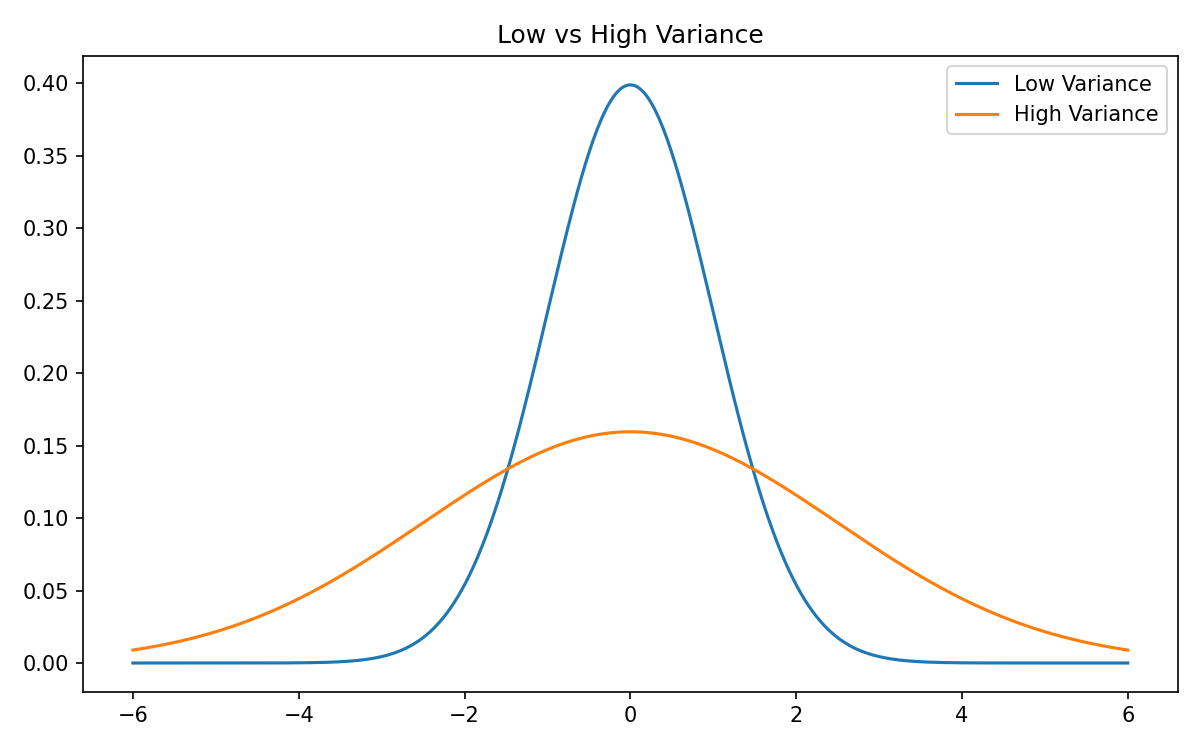
Variance: how wild the outcomes are

Variance measures how far outcomes tend to be from the mean:

$$\text{Var}(X) = \mathbb{E}[(X - \mu)^2]$$

Standard deviation: $\sigma = \sqrt{\text{Var}(X)}$.

High variance strategies:

• big swings
• long losing streaks
• deep drawdowns
• emotionally intense

Low variance strategies:

• smoother curves
• shallower drawdowns
• easier to stick with

Variance does not change expected value. It changes the experience of realizing that expected value.

In trading:

• Same EV, higher variance → more pain, more risk of ruin.
• This is why “path” matters as much as “destination.”

Skewness: where the big moves live

Skewness captures asymmetry — whether the distribution has heavier extremes on one side.

Mathematically:

$$\text{Skew}(X) = \frac{\mathbb{E}[(X - \mu)^3]}{\sigma^3}$$

Intuition:

Negative skew

• Many small wins

• Rare, large losses

• Feels smooth and comfortable… until a crash

• Typical of:

  • selling options
  • carry and yield strategies
  • grid/martingale-like systems

Positive skew

• Many small losses

• Rare, very large wins

• Feels frustrating and “wrong” most of the time

• Typical of:

  • trend following
  • convex payoff structures
  • lottery-like payoffs, tail hedging

Skew doesn’t change EV either — it changes how you earn that EV.

Your skew determines your emotional journey:

• Negative skew → long periods of comfort, rare trauma
• Positive skew → frequent discomfort, rare euphoria

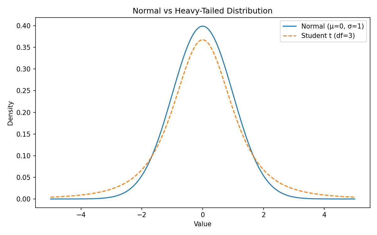
Kurtosis: how often extreme events happen

Kurtosis measures tail thickness — how common extreme outcomes are.

One convenient way to think about it:

• Low kurtosis (thin tails): extremes are rare
• High kurtosis (fat tails): extremes are common

Mathematically (excess kurtosis):

$$\text{Kurtosis}(X) = \frac{\mathbb{E}[(X - \mu)^4]}{\sigma^4}$$

In practice:

• Markets have fat tails: crashes, gaps, panics, liquidity cascades.
• These happen far more often than a normal distribution predicts.

In a normal model:

• a 5σ or 6σ event is “nearly impossible.” In markets:

• multi-sigma-type moves happen every decade or so.

Ignoring fat tails is how you get blindsided.

Why the normal distribution is only a starting point

The normal distribution is beloved in textbooks because it’s:

• symmetric
• fully determined by mean and variance
• analytically convenient

Under a normal assumption:

• returns cluster nicely around the mean
• tail events are extremely rare
• many formulas become simple

But real market return distributions typically show:

• skew (often negative)
• fat tails
• volatility clustering (high-volatility days follow high-volatility days)
• regime shifts
• jumps/gaps

So the normal distribution is useful as a baseline, but dangerous as a truth model.

Market distributions are non-stationary (they change over time)

Another crucial fact:

Market distributions drift. They are not fixed.

The distribution of returns:

• during a calm bull market
• during a panic selloff
• during a sideways chop

…are not the same.

Quant terms: markets are non-stationary.

What changes?

• mean (drift)
• variance (volatility)
• skew (direction of big moves)
• kurtosis (tail thickness)

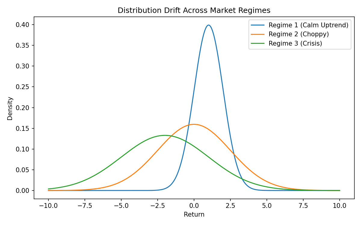
This is why:

• a strategy that worked in one regime can collapse in another
• backtests must span multiple regimes
• ongoing monitoring is critical

Discrete distribution example: more than just EV

Let’s consider a very simple discrete payoff:

Outcome	Probability
-1	0.5
+2	0.5

Expected value:

$$\mathbb{E}[X] = 0.5(-1) + 0.5(2) = 0.5.$$

Positive EV. Good game.

But the distribution tells us more:

• you lose half the time
• wins are larger than losses
• variance is high

So:

• you’ll often feel like you’re “wrong”
• but over many iterations, the edge dominates

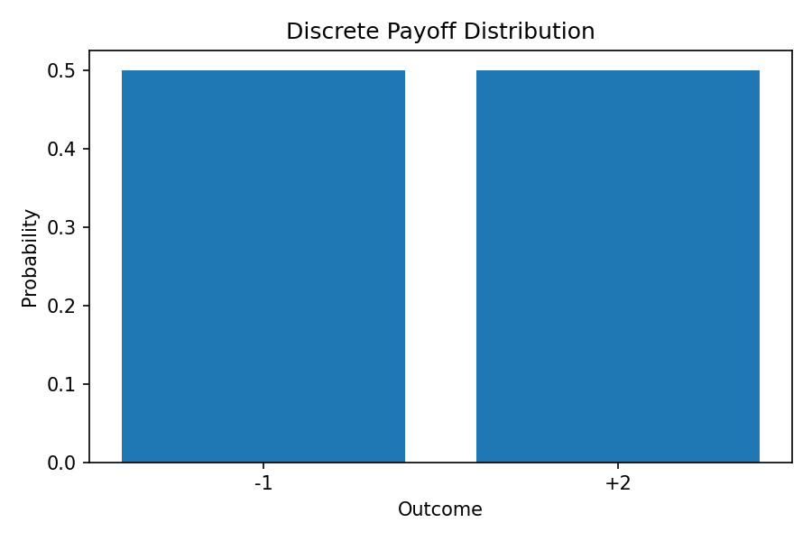
This small table already encodes:

• EV
• variance
• skew (positive — big wins)

Same EV, totally different distributions

Now compare two strategies with the same expected value, but different shapes.

Strategy A — Negative Skew

• Win $10 with 95% probability
• Lose $200 with 5% probability

Expected value:

$$\mathbb{E}[A] = 0.95(10) + 0.05(-200) = 9.5 - 10 = -0.5.$$

This one is actually negative EV, but let’s conceptually adjust numbers so both have similar EV. The key idea is shape:

• Many small wins
• Occasional large loss
• Feels great… until blowup

Strategy B — Positive Skew

• Lose $15 with 90% probability
• Win $150 with 10% probability

Expected value:

$$\mathbb{E}[B] = 0.9(-15) + 0.1(150) = -13.5 + 15 = 1.5.$$

• Frequent small losses
• Occasional large win
• Feels uncomfortable, but can be robust

Even when EVs are matched, the distributions:

• produce different drawdown profiles
• demand different psychology
• have different ruin probabilities

Distribution shape is often the difference between:

• “this strategy feels easy but dies suddenly”
• “this strategy is hard but survives.”

Distributions and emotional difficulty

Your strategy’s distribution directly shapes your emotional experience:

• Positive skew → many losing days, rare big wins

  • You will doubt yourself constantly.

• Negative skew → many winning days, rare disasters

  • You will feel like a genius, then suddenly ruined.

• High variance → long losing streaks, deep swings

• Low variance → smoother PnL, but may hide tail risk

If your psychology does not match your distribution, you will abandon the system, even if it is mathematically sound.

Understanding your distribution is understanding your lived reality as a trader.

Why traders must understand distributions

Distributions determine:

1. How long losing streaks can be
2. How deep drawdowns can get
3. How likely tail events are
4. How volatile your equity curve will feel
5. How robust your edge is under noise
6. Whether you can emotionally stick with the strategy

Expected value tells you the “center.” Probability distributions tell you the shape around that center.

And in real trading, the shape is often more important than the center.

Where we go next

We’ve talked about the shape of uncertainty. Next, we zoom into one key part of that shape:

How wide are the outcomes? How wild are the swings?