Mathematics of Trading: Modeling Randomness

Random Walks → Brownian Motion → Geometric Brownian Motion → Monte Carlo Simulation

How Markets Generate Noise, How We Model It, and Why Every Trading Strategy Exists Inside a Cloud of Possible Futures

Financial markets look noisy and chaotic:

• prices wiggle unpredictably
• shocks appear out of nowhere
• paths diverge dramatically
• volatility comes in clusters
• trends emerge and collapse

To understand:

• edge
• variance
• drawdowns
• ruin
• tail events
• strategy testing
• stress scenarios

we must understand randomness.

This post shows:

1. How randomness is modeled mathematically
2. How prices evolve in uncertain environments
3. Why Brownian motion is the backbone of modern finance
4. Why GBM is the standard model for price dynamics
5. Why Monte Carlo simulation is essential for real-world risk analysis

This is the most mathematically important post so far.

Randomness: The Foundation of Market Behavior

Markets look random even when they aren’t purely random.

They are driven by complex forces:

• order flow
• liquidity pressure
• news shocks
• behavioral cascades
• algorithmic interactions

Even so, randomness provides a tractable mathematical framework that captures essential features of market movement.

We begin with the simplest model.

Random Walks: The First Market Model

A random walk evolves by adding random increments:

$$X_{t+1} = X_t + \varepsilon_t$$

Where:

$$\varepsilon_t \sim {-1, +1}$$

A random walk captures:

• short-term unpredictability
• long-term variance growth
• path dependence
• divergence between sample paths

Variance grows linearly

$$\text{Var}[X(t)] = t\sigma^2$$

Meaning:

• uncertainty increases with time
• small randomness accumulates into large randomness

Distribution approaches normal

$$X(t) \approx \mathcal{N}(\mu t,\ \sigma^2 t)$$

even if the step distribution is simple.

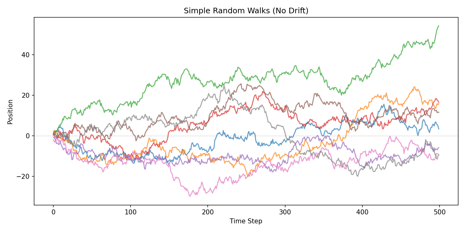
Random walks already look surprisingly like real markets.

But prices cannot go negative — that requires refinement.

Random Walks With Drift

Markets exhibit long-term upward drift (risk premium).

We add a deterministic trend:

$$X_{t+1} = X_t + \mu + \varepsilon_t$$

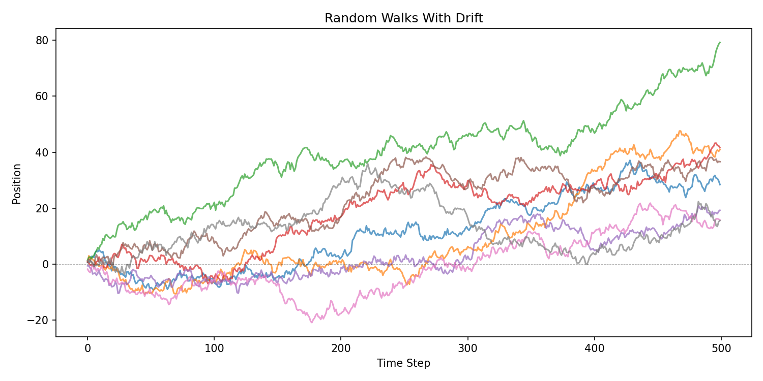
Now the process trends upward on average, but remains unpredictable path-by-path.

Still, this model is additive — markets are multiplicative.

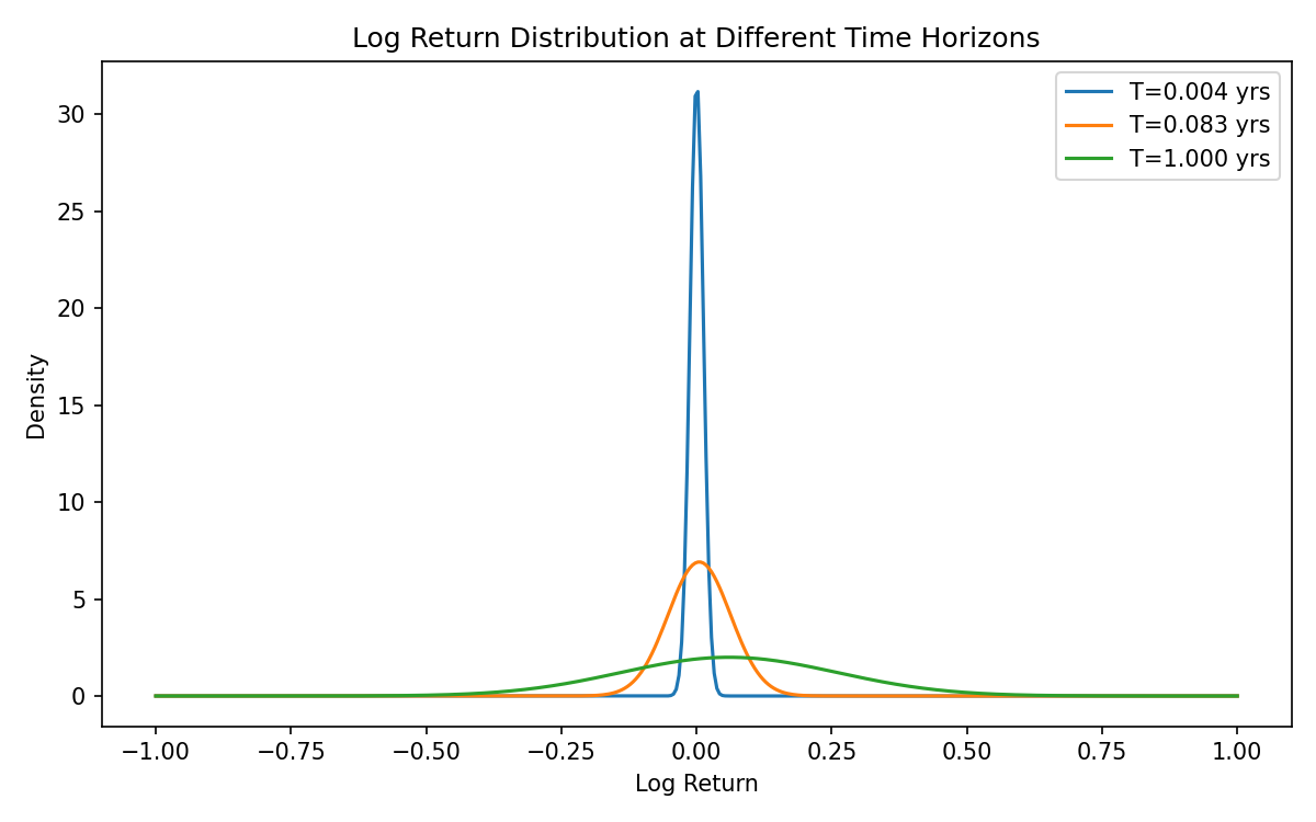
Log Returns: Fixing the “Negative Price” Problem

Markets move in percentages, not points.

• A 1% move at 100 = +1
• A 1% move at 200 = +2

So price changes scale with price.

We model log returns:

$$r_t = \ln\left(\frac{S_{t+1}}{S_t}\right)$$

Log returns are:

• additive
• stable
• symmetric-ish
• always yield positive prices

If log prices follow a random walk:

$$\ln S(t) = \ln S(0) + \mu t + \sigma W(t)$$

then prices are always positive.

Brownian Motion: Continuous-Time Randomness

Discrete random walks converge to a continuous-time stochastic process:

$$W(t)$$

Brownian motion (also called Wiener process).

Properties

1. ( W(0) = 0 )
2. Independent increments
3. Normal increments

$$W(t+\Delta t) - W(t) \sim \mathcal{N}(0,\Delta t)$$

4. Variance grows linearly:

$$\text{Var}[W(t)] = t$$

5. Continuous but nowhere differentiable (capturing jagged market behavior)

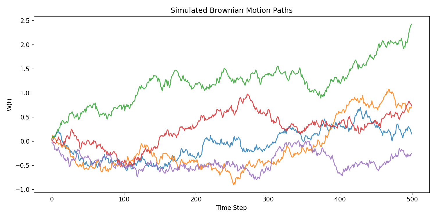
Brownian motion is the mathematical engine of nearly all classical financial modeling.

Brownian Motion With Drift

Add deterministic growth:

$$dX(t) = \mu,dt + \sigma,dW(t)$$

Interpretation:

• $\mu dt$: predictable drift
• $\sigma dW(t)$: stochastic noise

This structure maps directly to short-term unpredictability + long-term trend.

Geometric Brownian Motion (GBM): The Standard Model for Asset Prices

Raw Brownian motion can go negative — unacceptable for prices.

GBM fixes this:

$$dS(t) = \mu S(t), dt + \sigma S(t), dW(t)$$

This implies:

$$S(t) = S(0) \exp\left((\mu - \tfrac{1}{2}\sigma^2)t + \sigma W(t)\right)$$

Consequences

• prices stay positive
• log returns are normal
• volatility scales as $\sigma\sqrt{t}$
• paths diverge exponentially
• uncertainty grows multiplicatively

GBM is used in:

• Black–Scholes
• VaR models
• forecasting tools
• Monte Carlo simulators
• quantitative trading research

It is not perfect — but it is the essential baseline.

GBM vs Real Markets: Where the Model Breaks

GBM assumes:

• constant volatility
• no jumps
• normal returns
• no clustering
• no skewness
• no fat tails

Real markets have:

• volatility clustering
• fat tails
• negative skew
• jumps
• regime shifts
• autocorrelation in volatility

GBM is the starting point. Monte Carlo is how we test deviations from it.

Monte Carlo Simulation: Modeling Thousands of Futures

A single historical backtest gives one path.

Monte Carlo simulation gives thousands.

It answers:

• How wide is the distribution of possible outcomes?
• How deep can drawdowns get?
• How frequently does ruin occur?
• How much tail risk exists?
• How volatile is performance across paths?

Monte Carlo = risk in full resolution.

Monte Carlo Example Set 1 — Gambling Games

Example A: Coin Flip Wealth Paths

Game:

• +1 for heads
• –1 for tails
• 200 flips

Simulate 10 paths.

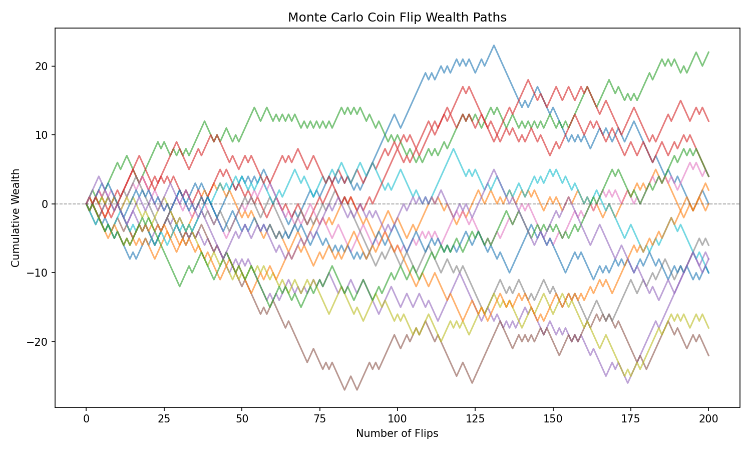
Observations:

• same rules, wildly different outcomes
• variance compounds
• prediction is impossible

Example B: Gambler’s Ruin

Start with $100 Bet$1 per flip Goal: reach $200 Ruin: reach$0

Monte Carlo estimates:

• probability of ruin
• distribution of time to ruin
• expected play length
• impact of unfavorable odds

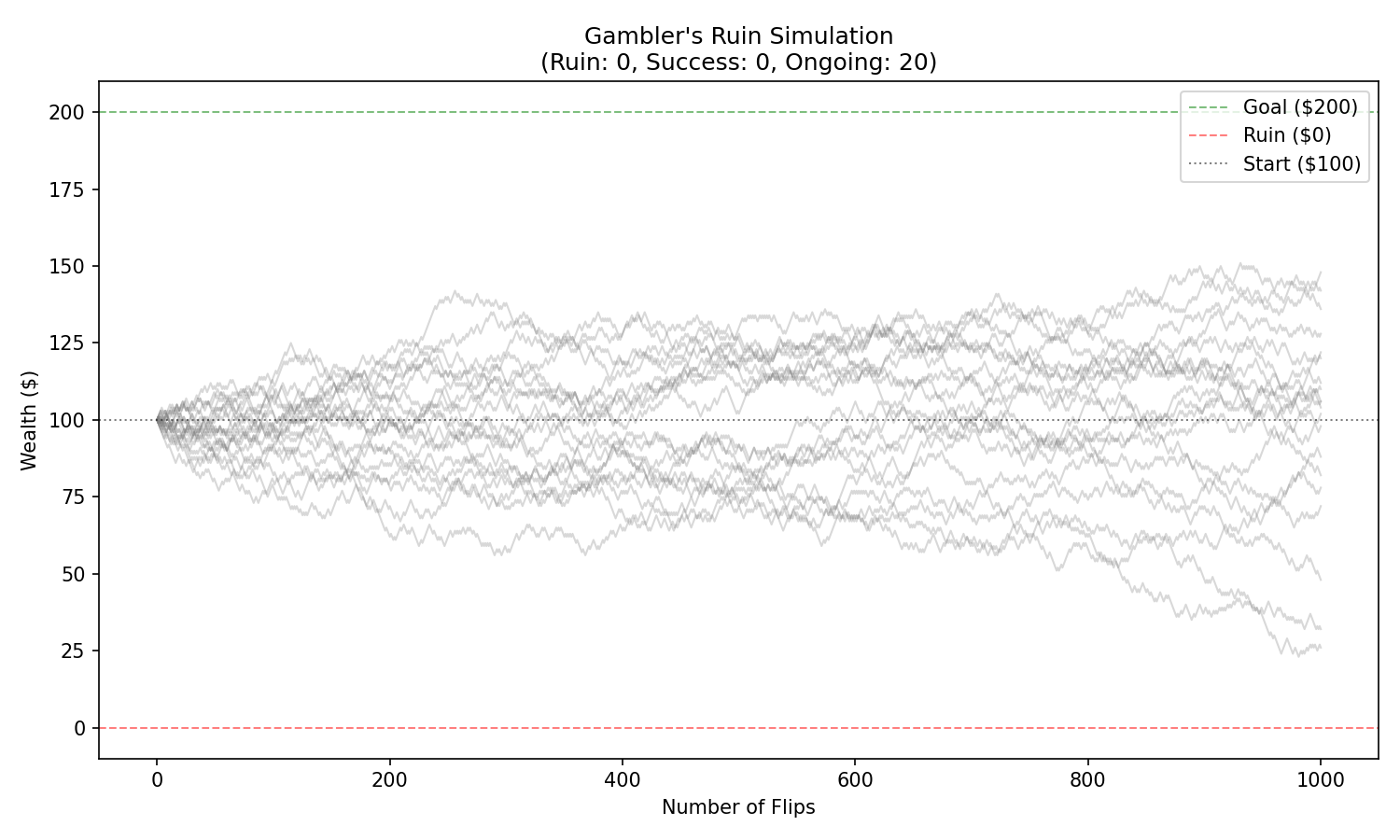
This problem is the ancestor of modern risk-of-ruin theory.

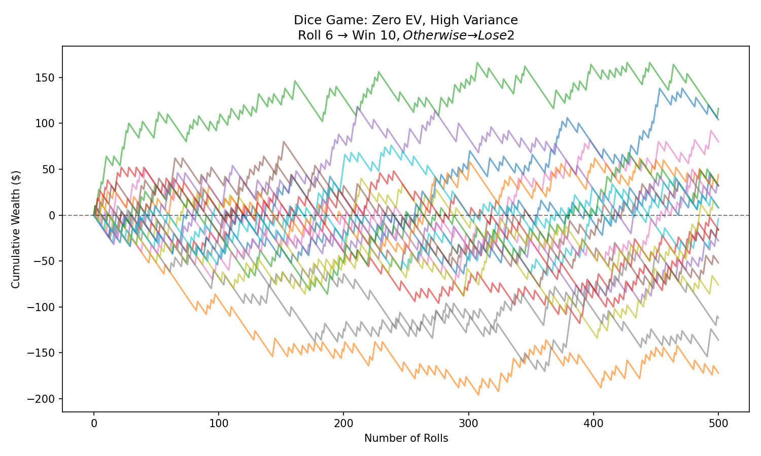
Example C: Dice Game EV Simulation

Game:

• roll a die
• 6 → win $10
• otherwise → lose $2

Analytical EV = 0

But Monte Carlo shows:

• long drawdowns
• variance around 0
• risk of ruin despite fair odds

11. Monte Carlo Example Set 2 — Markets

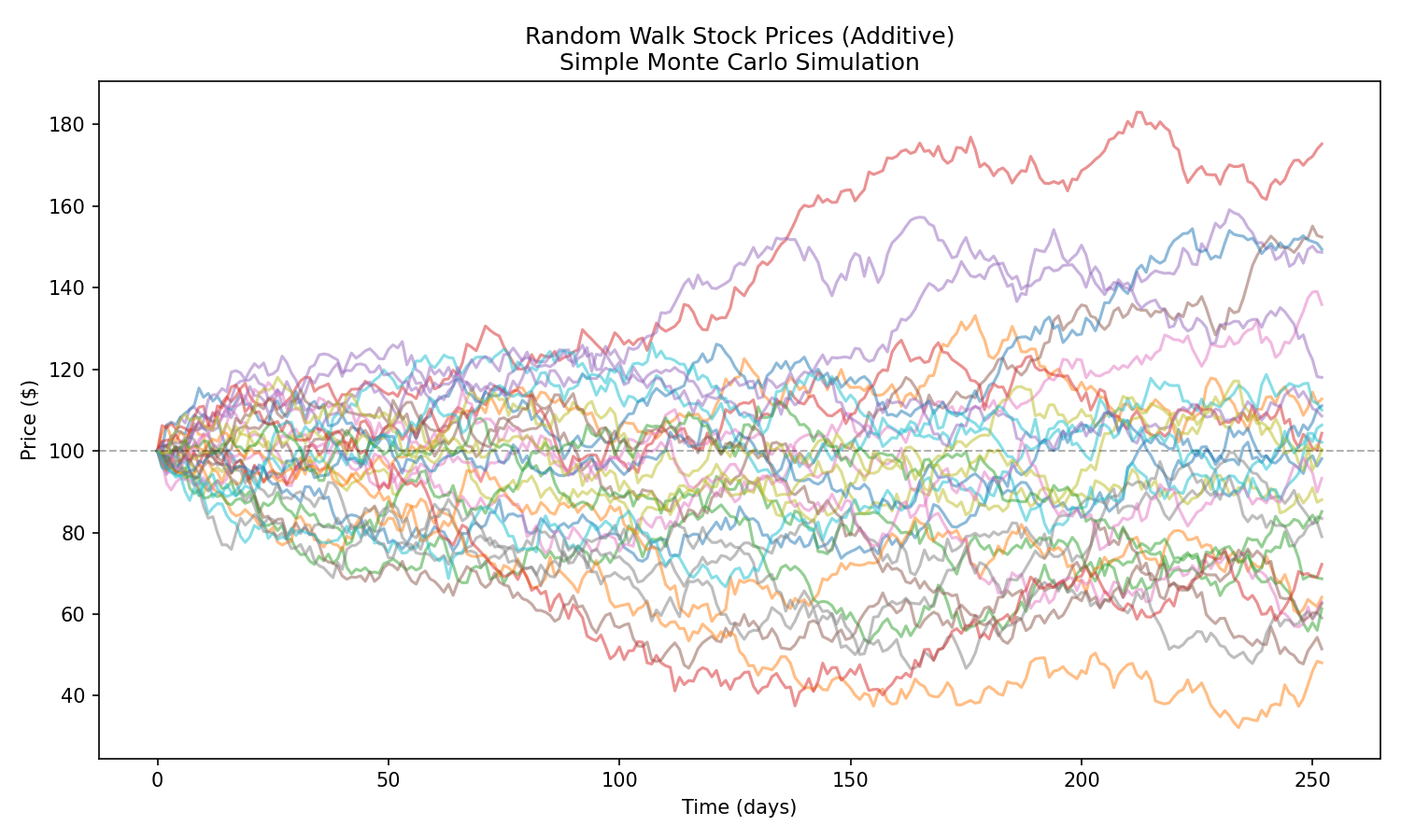
A. Random Walk Stock Prices

The simplest price simulation.

Reveals:

• range of possible trajectories
• divergence of sample paths
• exploding uncertainty over time

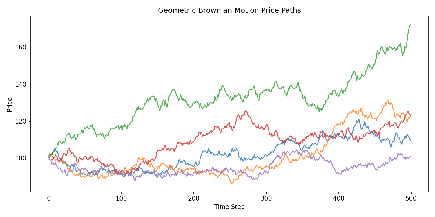
B. GBM Price Simulations

For GBM:

$$S_{t+1} = S_t \exp\left((\mu - \tfrac12\sigma^2)\Delta t + \sigma\sqrt{\Delta t}Z_t\right)$$

with $Z_t \sim \mathcal{N}(0,1)$.

Simulate 50 paths:

• drift nudges upward
• volatility broadens the cone
• uncertainty grows exponentially
• extreme paths appear naturally

C. Final Price Distributions

Simulate 10,000 paths.

Ending prices follow a log-normal distribution:

• median < mean (volatility drag)
• fat right tail
• left skew from price floor at 0

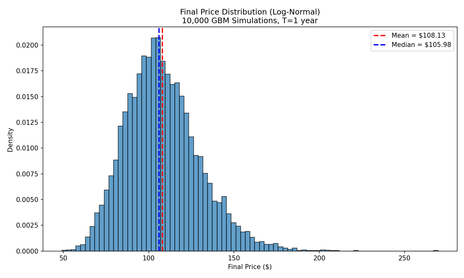
This distribution underlies:

• Black–Scholes
• geometric mean return
• exponential wealth dynamics

D. Strategy Return Bootstrapping

Let strategy returns follow some empirical distribution.

Simulate equity curves:

$$Equity_{t+1} = Equity_t (1 + r_t)$$

Repeating thousands of times reveals:

• expected drawdown
• 95% worst-case drawdown
• variability of Sharpe ratio
• likelihood of different future paths

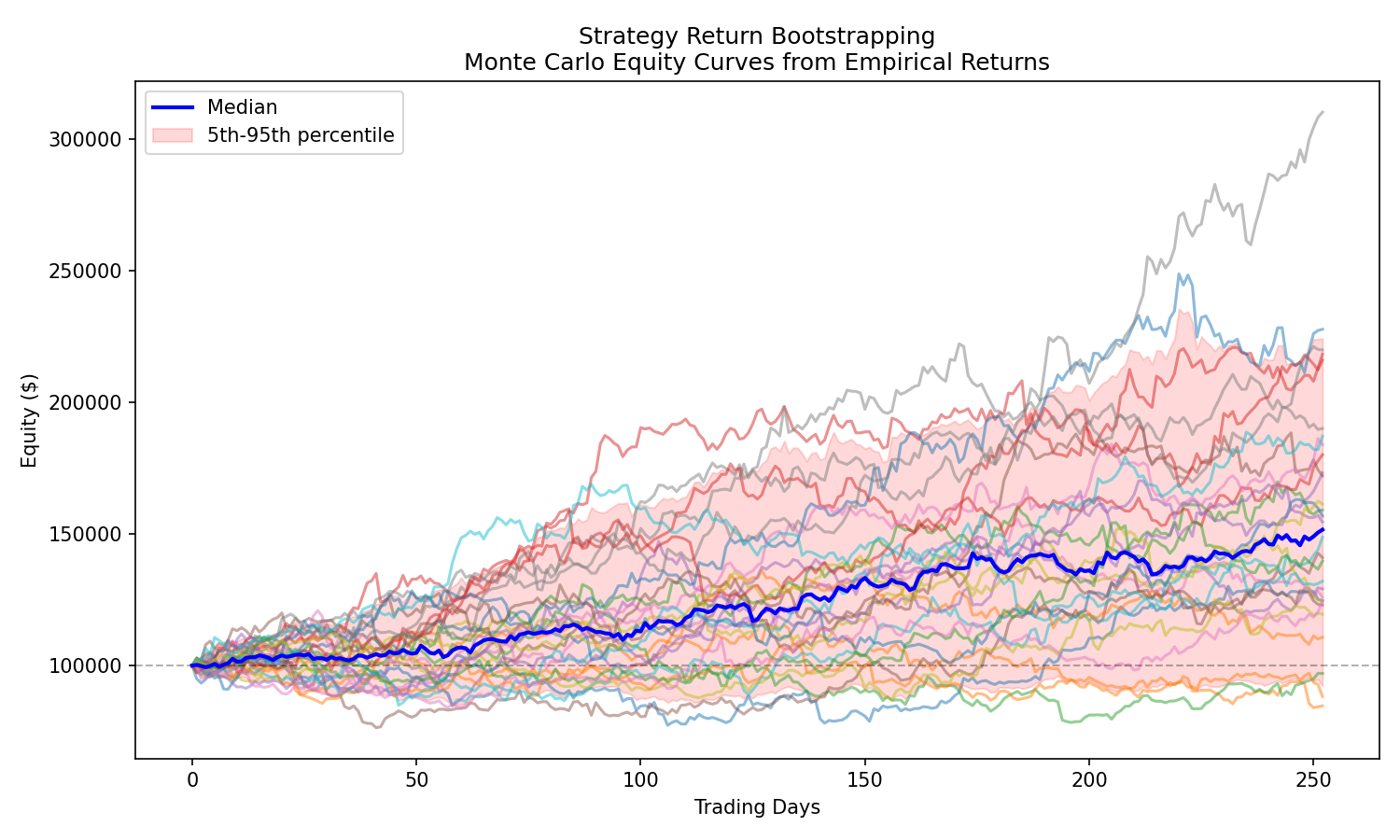
No single backtest can reveal this.

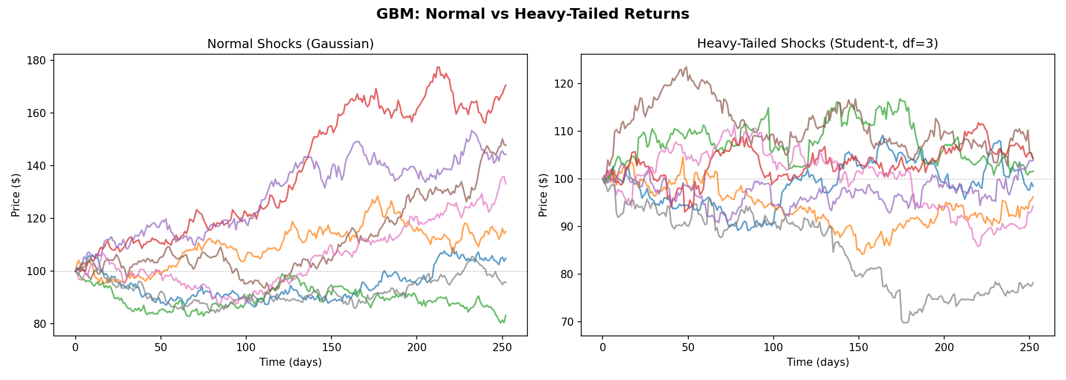
E. Heavy-Tailed Crash Scenarios

Replace normal shocks with Student-t shocks:

$$Z_t \sim t(\nu)$$

This introduces:

• more crashes
• fatter tails
• more ruin events
• more realistic crisis dynamics

F. Forecast Cones (Fan Charts)

Compute percentiles across paths:

• 5th percentile (worst case)
• median
• 95th percentile (optimistic)

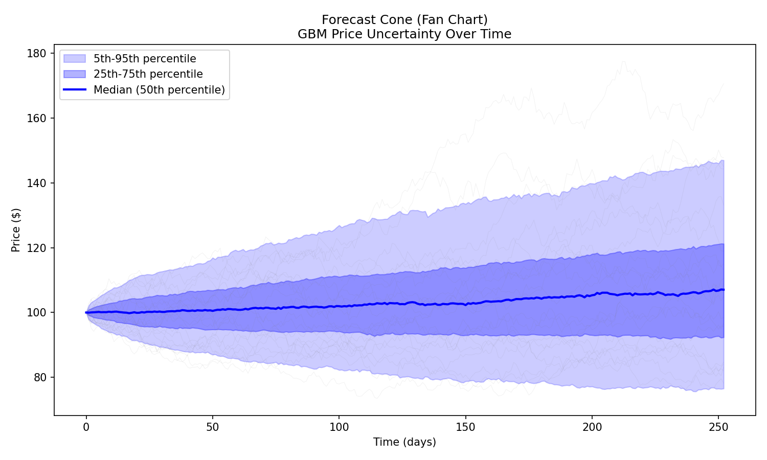
This creates the "uncertainty cone" used in:

• portfolio management
• risk reporting
• long-term forecasting

Why Monte Carlo Is Essential

Backtesting answers:

Does this system work on one historical path?

Monte Carlo answers:

Does this system survive thousands of plausible futures?

Monte Carlo exposes:

• hidden fragility
• left-tail danger
• sizing issues
• variance shock sensitivity
• survival probability
• robustness to noise
• drawdown uncertainty

Professional traders never deploy strategies without Monte Carlo analysis.

Key Takeaways

• Random walks are the base model of unpredictability

• Brownian motion is the continuous-time limit

• GBM ensures positivity & multiplicative returns

• Markets deviate from GBM but GBM is the essential baseline

• Monte Carlo simulation is the only way to understand:

  • drawdowns
  • ruin
  • performance variability
  • tail risk
  • robustness

Every trading strategy is not one equity curve. It is a distribution of equity curves.

Monte Carlo lets you see that distribution.